Chapter 5 Spatial Analysis

In order to visualize our data and perform spatial analysis we will import the clustering results into CODEX MAV.

5.1 Annotate Populations

Open imageJ and launch CODEX MAV. Open the experiment and select No Clustering (Figure 28). Import Seurat clusters by selecting File -> Import clustering run and open the folder named clusters_compensated. When prompted, accept the folder as correct and select cluster_ID as the column to identify clusters (Figure 28).

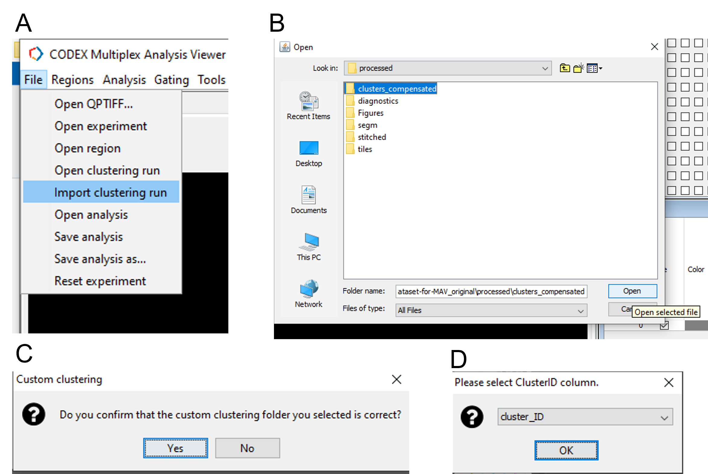
Figure 28. Import clusters into CODEX MAV.

The clusters will appear in the clustering tab of CODEX MAV. In order to visualize the clustering annotations on cells add the clusters to the populations table. You may use the add or add All button. We recommend using the Add button (blue arrow, Figure 29).

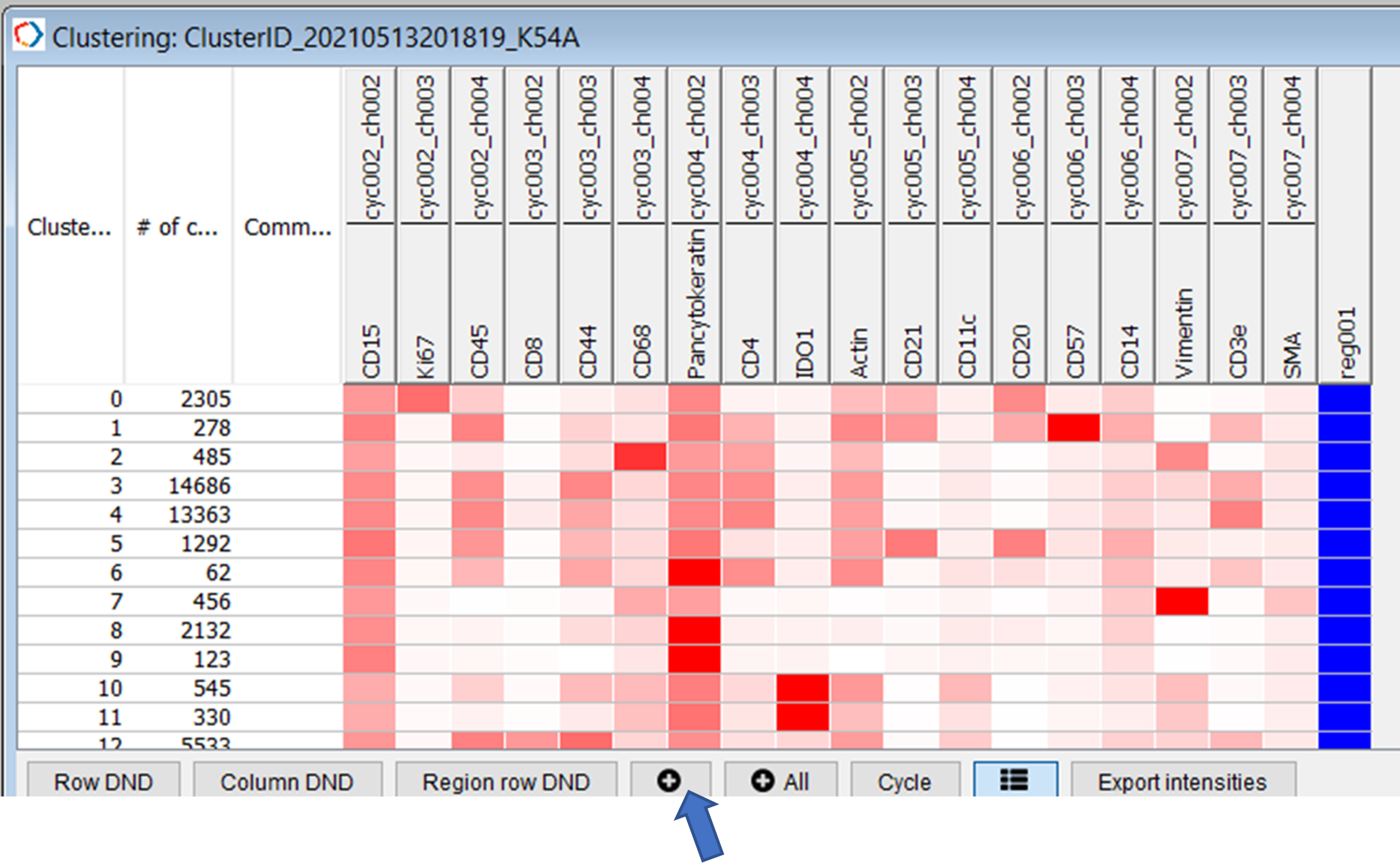
Figure 29. Add Seurat clusters as populations.

After clusters have been added as populations and annotated (click on population name to annotate) you may color populations by dendrogram similarity (Figure 30).

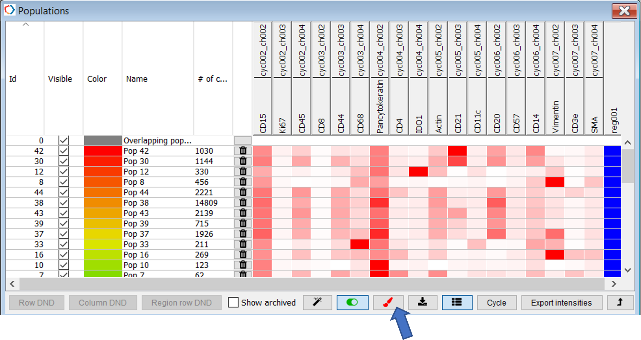
Figure 30. Populations table in Main window. Click paintbrush to color by dendrogram similarity.

5.2 Calculate spatial proximities

To calculate spatial relationships between the annotated populations, tick the checkbox for populations of interest in the populations window. Navigate to Analysis -> Spatial analysis -> All regions -> specify max distance (30 microns is a good starting point) -> select OK (Figure 31).

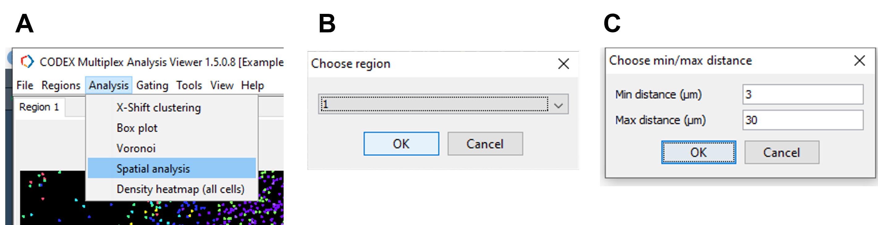
Figure 31. Calculate log odds ratio for spatial proximity analysis in CODEX MAV

In the resulting table, red colored populations are likely to be found within the set proximity while blue colored populations are unlikely to be found within the set proximity (30 microns, Figure 32).

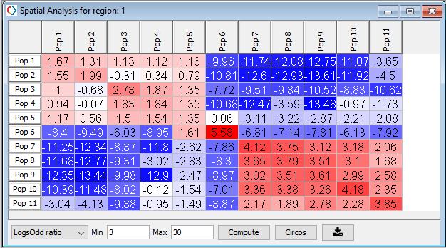
Figure 32. Spatial proximity analysis showing log odds ratio