Chapter 4 Implementation of Seurat Analysis

In this section we will review how to run the Seurat analysis. Subsequent sections will explain individual parts of the code. This section is dedicated to running the code.

4.1 Save scripts and set paths

Download STEP_part_1 and save it to C:/Users/(insert user name).

There are three files that need to be downloaded for STEP analysis. The first file is a python script called neighbors.py. This file needs to be saved to C:/Users/(insert user name).

Next, download STEP_part_2. Save the file to C:/Users/(insert user name).

Open STEP_part_2.Rmd by double clicking on the file. Scroll down to line 334. You will see a chunk of code that looks like:

############################# USER INPUT REQUIRED ##############################
#Chunk 4
#source_python("C:\\Users\\(user name)\\neighbors.py")#line 334 of STEP_part_2
################################################################################

In Windows my user name is gcarlson as shown in Figure 12. So line 334 of STEP_part_2 becomes:

############################# USER INPUT REQUIRED ##############################
#Chunk 4
#source_python("C:\\Users\\gcarlson\\neighbors.py")#line 334 of STEP_part_2
################################################################################

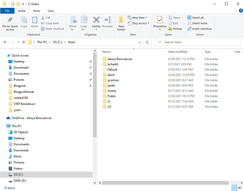
Figure 12. Example of Windows username.

On line 18 of STEP_part_1 update the path so that it points to STEP_part_2 as shown below:

#Chunk 1
#Open packages required for use
#install.load::install_load('reticulate','plyr', 'openxlsx', 'readxl', 'magrittr', 'purrr', 'ggplot2','Seurat', 'tidyverse', 'patchwork', 'dplyr', 'BiocManager', 'cowplot', 'svDialogs', 'knitr')

#use_condaenv("neighborhood")

#path="C:\\Users\\gcarlson\\STEP_part_2.Rmd" # This is line 18 of STEP_part_1

4.2 Configure Anaconda 3 conda environment

Open Anaconda Prompt (Figure 13). 

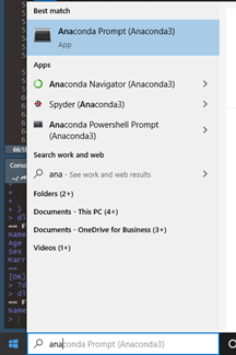
Figure 13. Open Anaconda Prompt.

Create a new environment called neighborhood (Figure 14) by typing conda create –name neighborhood. 

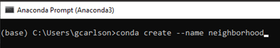
Figure 14. Create conda environment called neighborhood.

Activate the conda environment by typing conda activate neighborhood (Figure 15).

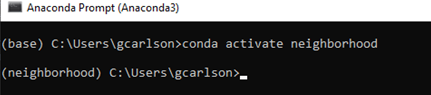
Figure 15. Activate conda environment.

Install conda packages by typing conda install pandas numpy matplotlib seaborn (Figure 16).

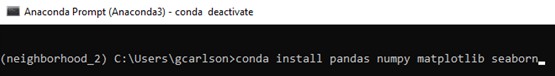
Figure 16. Install packages and modules.

When prompted to proceed enter y to proceed (Figure 17).

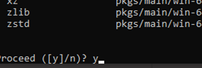
Figure 17. When prompted to proceed enter y.

Install pip packages by typing pip install sklearn pathlib easygui (Figure 18).

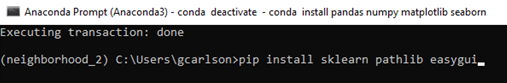
Figure 18. Install packages via pip.

4.3 Run STEP Analysis

To run the STEP analysis, update the working directory by specifying setwd(C:/Users/user name) click Run and Run All as shown in Figure 19.

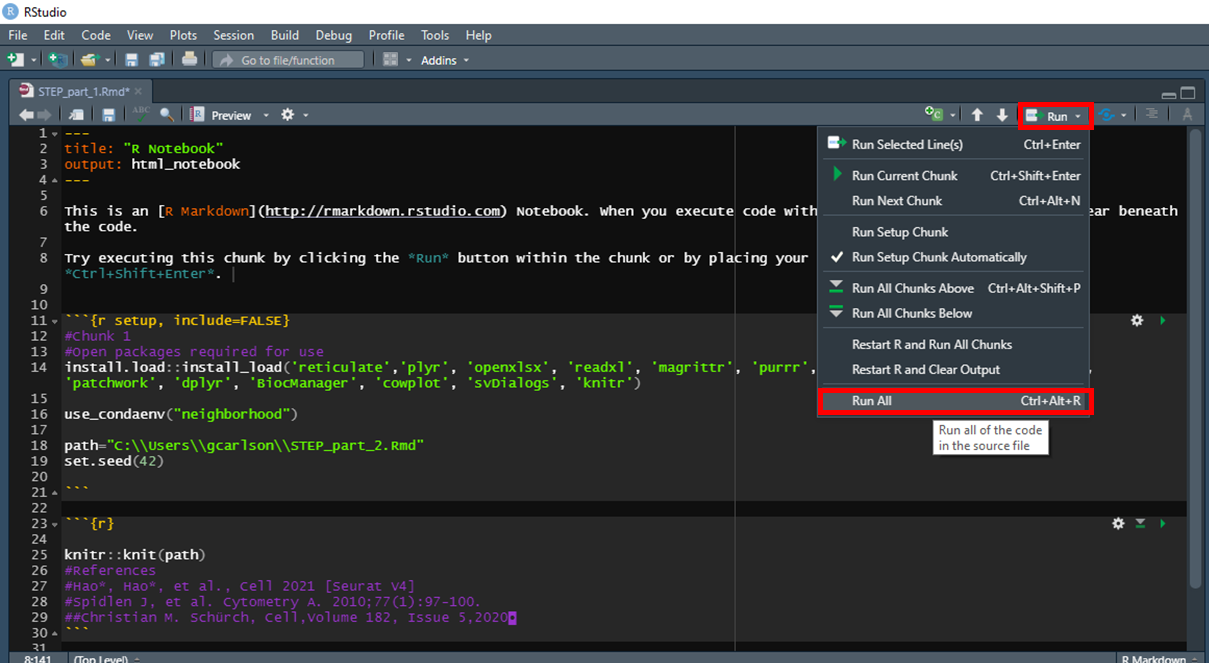
Figure 19. Example of Windows username.

Upon prompt, specify the directory of the cell segmentation data. For CODEX MAV experiment cell segmentation data are always saved in processed/segm/segm-1/fcs/compensated as shown in Figure 20.

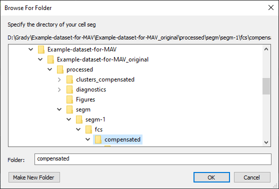
Figure 20. Select directory of cell segmentation data.

Next, you will receive a prompt to enter the name of the saved analysis state. Type in the name of the saved analysis state and click OK (Figure 21).

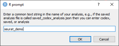
Figure 21. Type the name of the saved analysis state and click OK.

On prompt, enter the number of spatial neighbors to define the size of the spatial window. It is recommended to start with 20 neighbors. This number must always be greater than the number of cell neighborhoods (Figure 22).

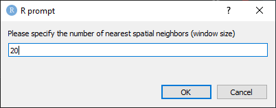
Figure 22. Enter the number of spatial neighbors to define the size of the spatial window.

Next, specify the number of cell neighborhoods. It is recommended to start with 10 neighborhoods if working with greater than 30 markers. Smaller panels may warrant fewer neighborhoods (Figure 23).

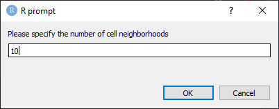
Figure 23. Specify the number of cell neighborhoods.

The analysis produces Figures for UMAP, cluster heatmap, ridgeplots (histograms), and cell neighborhood heatmap. All figures are written to the directory processed/Figures.

4.4 Figures

4.4.1 UMAP

Seurat allows us to calculate UMAP or tSNE. In this example, we calculate UMAP. The goal of these dimensional reduction algorithms is to learn the underlying manifold of the data in order to place similar cells together in low-dimensional space. Cells within the graph-based clusters determined above should co-localize on these dimension reduction plots.UMAP plots can be displayed with clusters (Figure 24) or features (Figure 25).

Figure 24. UMAP Plot overlaid with clusters

Plotting UMAP with features is one visual aid in a series of tools that helps us to determine cell phenotypes in tissue. UMAP feature plots help to visualize and identify broad classes of phenotypes, i.e., epithelial, T-cell, B-cell, etc… Colocalized cells are most similiar.

### Heatmap The Seurat heatmap is a useful tool for identification of distinct cell populations and phenotypes. Yellow lines indicate relatively high expression of antigen and purple lines indicate relatively low or no expression of antigen. Frequency of cell expression is indicated by the number of purple, black, or yellow lines (Figure 26). If after viewing the heatmap it is unclear whether two populations have similar expression of target antigen, we recommend to inspect the antigen expression in the ridgeplot (Figure 27).

### Ridgeplot The ridgeplot provides a more granular view of the frequency and intensity of antigen expression for cells within in each cluster. For each antigen, clusters are plotted in order of increasing antigen expression, such that the last cluster (bottom most) plotted contains cells with the greatest antigen expression.

We will annotate clusters after we import them back into CODEX MAV.